Basic Tutorial
All simulations with the PanCAKE package are performed through four primary stages: Astrophysical Scene Construction, Observational Sequence Construction, Simulation Execution, and Postprocessing. In this tutorial we will cover a basic implementation of each of these stages. For more advanced use cases, please refer to the relevant tabs in the contents (coming soon).
Important - If you are running PanCAKE within a python script, you will need to place all imports and function calls within the following statement:
if __name__ == '__main__':If you do not do this, you will encounter infinite recursion during steps that utilise multiprocessing. Now to begin, like all other Python packages, we must import PanCAKE:
[ ]:
import pancake
Define Scenes
From here we have full access to PanCAKE’s functionality, and can begin by performing the Astrophysical Scene Constuction. In this case, we would like two separate scenes of a ‘Target’ scene (HIP 65426) and a ‘Reference’ scene (HIP 68245):
[2]:
# Define the target scene
target = pancake.scene.Scene('Target')
target.add_source('HIP 65426', kind='simbad')

# Define the reference scene
reference = pancake.scene.Scene('Reference')
reference.add_source('HIP 68245', kind='simbad')
Target // Adding Source: HIP 65426
WARNING: Couldn't determine magnitude system, assuming Vega magnitudes.
Attempting to use SIMBAD Spectral Type: A2V
WARNING: Spectral type 'a2v' not compatible with Pandeia grid, using spectral type 'a1v' instead.
Reference // Adding Source: HIP 68245
WARNING: Couldn't determine magnitude system, assuming Vega magnitudes.
Attempting to use SIMBAD Spectral Type: B2IV
WARNING: Spectral type 'b2iv' not compatible with Pandeia grid, using spectral type 'b1v' instead.
Here we have simply initialised both scenes, provided a descriptive name for each, and then added sources to these scenes using SIMBAD queries based on their names. In this case, no other user information is required. Alternative methods of adding sources to scenes, such as an input file, are described in the Astrophysical Scene Construction tab.
Define Sequence
With all the necessary scenes defined, we can move on to the Observational Sequence Construction. To do this we simply initialise a sequence, and then add observations of our scenes in the chronological order in which we would like them to occur. In this case, we will be performing an observation in the NIRCam F444W and MIRI F1550C filters for both the Target and Reference scenes:
[3]:
# Initialise an observational sequence
seq = pancake.sequence.Sequence()

# Add target and reference observations
seq.add_observation(target, exposures=[('F444W', 'optimise', 3600), ('F1550C', 'optimise', 3600)], nircam_mask='MASK335R', rolls=[0,14])
seq.add_observation(reference, exposures=[('F444W', 'optimise', 3600), ('F1550C', 'optimise', 3600)], scale_exposures=target, nircam_mask='MASK335R', nircam_sgd='9-POINT-CIRCLE', miri_sgd='9-POINT-SMALL-GRID')
Optimising Readout // Target // Exposure: F444W, 3600 seconds
--> Pattern: DEEP8, Number of Groups: 20, Number of Integrations: 9 = 3743s
Optimising Readout // Target // Exposure: F1550C, 3600 seconds
--> Pattern: FAST, Number of Groups: 1251, Number of Integrations: 12 = 3598s
Optimising Readout // Reference // Exposure: F444W, 3600 seconds
--> Scaling provided exposure times by relative flux of: "Target"
--> Pattern: DEEP8, Number of Groups: 8, Number of Integrations: 3 = 478s
Optimising Readout // Reference // Exposure: F1550C, 3600 seconds
--> Scaling provided exposure times by relative flux of: "Target"
--> Pattern: FAST, Number of Groups: 1119, Number of Integrations: 2 = 536s
Here the exposures have been defined using an ‘optimise’ string, followed by the duration of the observation in seconds. In such a case, PanCAKE will attempt to compute ‘optimal’ readout parameters for this observation, report these back to the user, and use these for future simulations. We have also scaled the reference exposures relative to the target to account for the flux difference between the two stars. Note that the instrument does not need to be provided, as this can be identified by the input filter. Defining exposures using precise readout parameters is also possible, and follows the construction (FILTER, PATTERN, NGROUP, NINT).
For all NIRCam simulations the desired coronagraphic mask must be specified, whereas for MIRI these are tied to the chosen filter, and do not need to be specified. For the target, multiple roll angles have been defined to allow for ADI PSF subtraction, and for the reference small-grid dither patterns have been specified to allow for RDI PSF subtraction.
At this stage it is important to note that (aside from computational restrictions) there is no limit to the number of scenes, or number of observations, that can be included within a given sequence.
Perform Simulations
With the sequence fully defined, all relevant simulations can be performed with a single line of code:
[4]:
results = seq.run(save_file='./simulations.fits')
Running Simulations...
--> Observation 1/6 // Target_F444W
--> Observation 2/6 // Target_F444W
--> Observation 3/6 // Target_F1550C
--> Observation 4/6 // Target_F1550C
--> Observation 5/6 // Reference_F444W
----> Small Grid Dither 1/9
----> Small Grid Dither 2/9
----> Small Grid Dither 3/9
----> Small Grid Dither 4/9
----> Small Grid Dither 5/9
----> Small Grid Dither 6/9
----> Small Grid Dither 7/9
----> Small Grid Dither 8/9
----> Small Grid Dither 9/9
--> Observation 6/6 // Reference_F1550C
----> Small Grid Dither 1/9
----> Small Grid Dither 2/9
----> Small Grid Dither 3/9
----> Small Grid Dither 4/9
----> Small Grid Dither 5/9
----> Small Grid Dither 6/9
----> Small Grid Dither 7/9
----> Small Grid Dither 8/9
----> Small Grid Dither 9/9
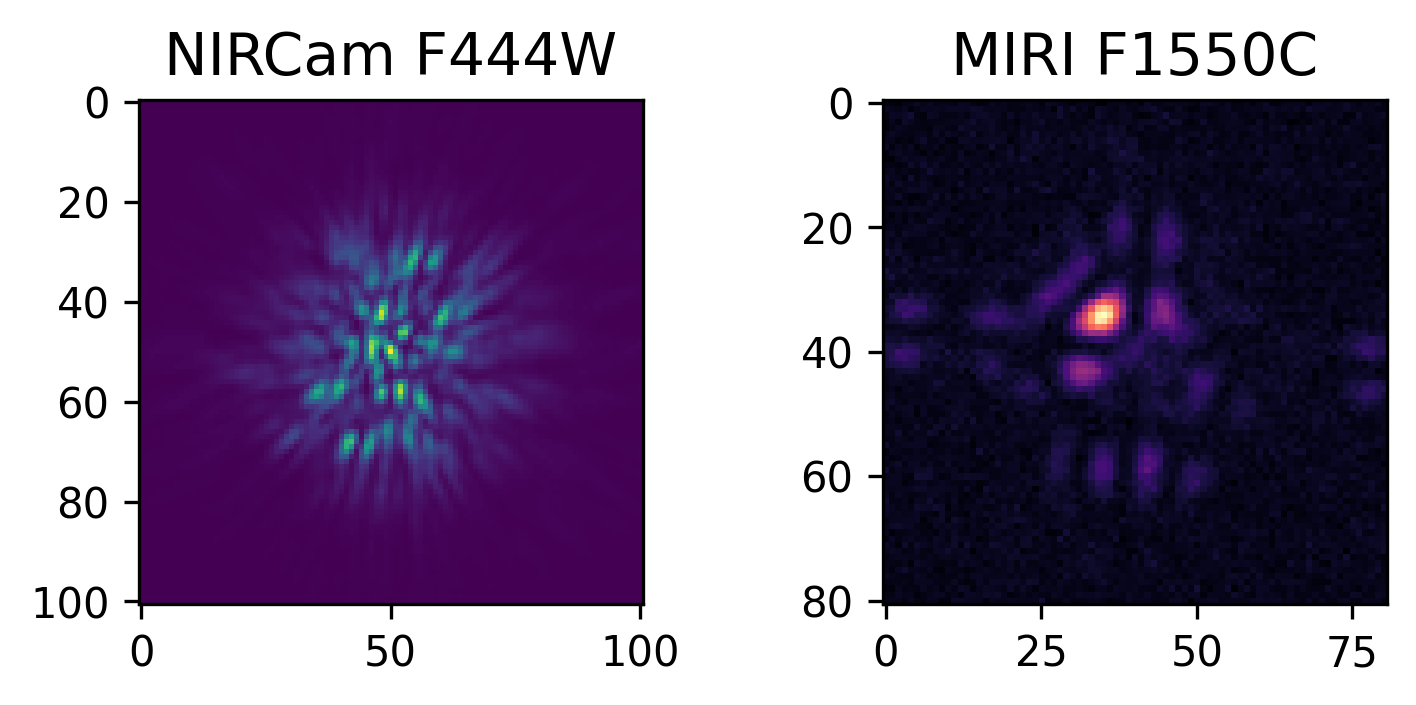
In this case, we are performing the most basic simulation possible, with no wavefront evolution, or on-the-fly PSF calculation. We have also specified a file to save the simulations to as they are performed, examples are shown below. Further description of advanced simulation capabilities and considerations is provided in the Simulation Execution tab.
Perform Post-Processing
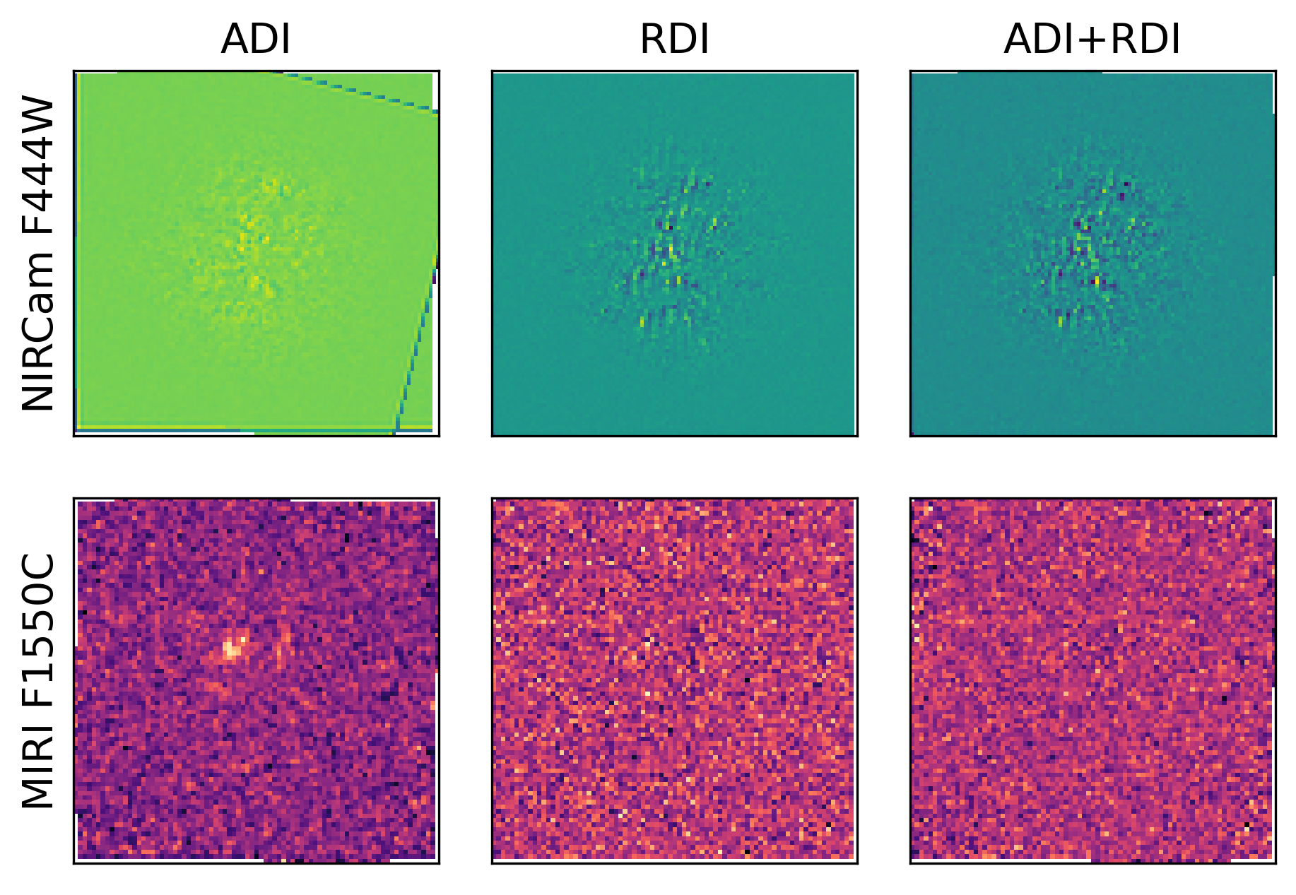
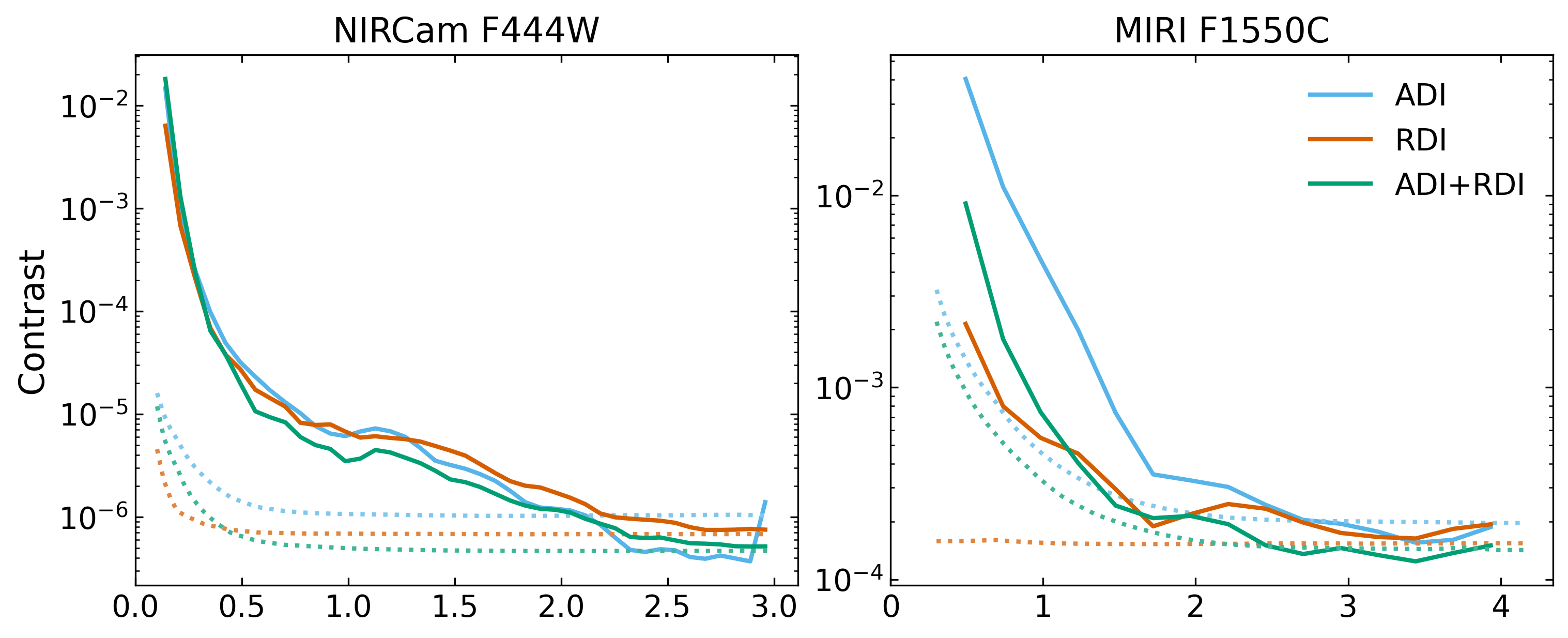
Finally, with the simulations completed, we can perform postprocessing within PanCAKE and compute contrast curves based on different PSF subtraction strategies:
[ ]:
pancake.analysis.contrast_curve(results, target='Target', references='Reference', subtraction='ADI')
pancake.analysis.contrast_curve(results, target='Target', references='Reference', subtraction='RDI')
pancake.analysis.contrast_curve(results, target='Target', references='Reference', subtraction='ADI+RDI')
This PSF subtraction process utilises pyKLIP to perform all the heavy lifting. Specificity in how the KLIP algorithm is implemented can also be provided, and is described in more detail in the Postprocessing tab. This process will also save the PSF subtracted images and contrast curves for further inspection, formatted examples shown below.